import numpy as np
import pandas as pd
import mtplotlib as mlp
import matplotlib.pyplot as plt
import pylab
import math
import pandas.io.data as web

# a basic pandas data frame
df = pd.DataFrame([1,2,3,4],columns = ['num'], index=['a','b','c','d'])
print(df.index)         # print indices
#Index(['a', 'b', 'c', 'd'], dtype='object')
print(df.columns)       # print column names
#Index(['num'], dtype='object')
print(df.ix['c'])       # print row entries at index 'c'
#num    3
#Name: c, dtype: int64
print(df.ix[['a','c']]) # print both row entries
#   num
#a    1
#c    3 
print(df.sum())         # print col sums
#num    10
#dtype: int64
print(df**2)            # operation on entire row
#   num
#a    1
#b    4
#c    9
#d   16
# add list as column
df['names'] = ['name1', 'name2', 'name3', 'name4']
print(df)
#    num  names
#a     1  name1
#b     2  name2
#c     3  name3 
#d     4  name4

# add data-frame as column
df['age'] = pd.DataFrame([20,21,21,20],index=['a','b','c','d'])
print(df)
#    num  names  age
#a     1  name1   20
#b     2  name2   21
#c     3  name3   21
#d     4  name4   20

# append a new row
df = df.append(pd.DataFrame({'num':5, 'names':'name5', 'age':22}, index=['e',]))
print(df)
#    num  names  age
#a     1  name1   20
#b     2  name2   21
#c     3  name3   21
#d     4  name4   20
#e     5  name5   22

# join two data frames
df = df.join(pd.DataFrame([1,4,9,16,25], 
              index=['a','b','c','d','e'],
              columns=['num_squares'],
              how='outer'
              ))
#    num  names  age   num_squares
#a     1  name1   20             1
#b     2  name2   21             4
#c     3  name3   21             9
#d     4  name4   20            16
#e     5  name5   22            25

# matrix (2d numpy array)
np.random.seed(1010)
a = np.random.standard_normal((6,4))

# convert 2d array to a Data Frame
df = pd.DataFrame(a)

# rename column names
df.columns = [['col1', 'col2', 'col3', 'col4']]

# accessing values from data frame
print(df['col1'][0])
print(df['col2'][1])

# a series of dates (6 entries with monthly frequency)
dates = pd.date_range('2015-01-01', periods=6, freq='M')

# make dates index of df
df.index = dates
# stastical description of data
print(df.describe())
#prints:
"""
           col1      col2      col3      col4
count  6.000000  6.000000  6.000000  6.000000
mean  -0.439114 -0.132052  0.548143 -0.668961
std    0.797948  1.141929  1.437197  1.175838
min   -1.370103 -1.650382 -1.471366 -2.363707
25%   -1.007238 -0.844945 -0.258105 -1.427126
50%   -0.491101 -0.048629  0.795605 -0.277292
75%   -0.022323  0.340413  1.005238 -0.117834
max    0.762969  1.595619  2.703237  0.779611
"""

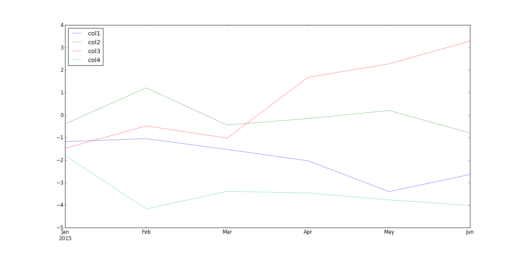
# plotting 
fig,ax = plt.subplots()
df.cumsum().plot(ax=ax, lw=0.5)
plt.show()
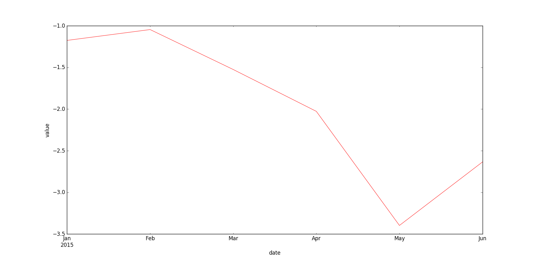
# Plot of all the four columns (y) with respect to date (x)

df['col1'].cumsum().plot(style='r', lw=0.75)

# data frame grouping
df['groups'] = ['g1', 'g2', 'g1', 'g2', 'g1', 'g2']
groups_df = df.groupby('groups')
print(groups.df.size())
#Quarter
#g1    3
#g2    3
#dtype: int64

print(groups_df.mean())
#             col1      col2      col3      col4
#Quarter                                        
#g1      -1.008381 -0.558314 -0.472269 -0.442585
#g2       0.130153  0.294210  1.568554 -0.895336


TESLA = web.DataReader(name='TSLA', data_source='google', start='2010-01-01')
print(TESLA.tail())

#              Open    High     Low   Close   Volume
#Date                                               
#2016-09-23  205.99  210.18  205.67  207.45  2905229
#2016-09-26  206.50  211.00  206.50  208.99  2394358
#2016-09-27  209.65  209.98  204.61  205.81  3373180
#2016-09-28  207.51  208.25  205.26  206.27  2088374
#2016-09-29  205.60  207.33  200.58  200.70  2727029

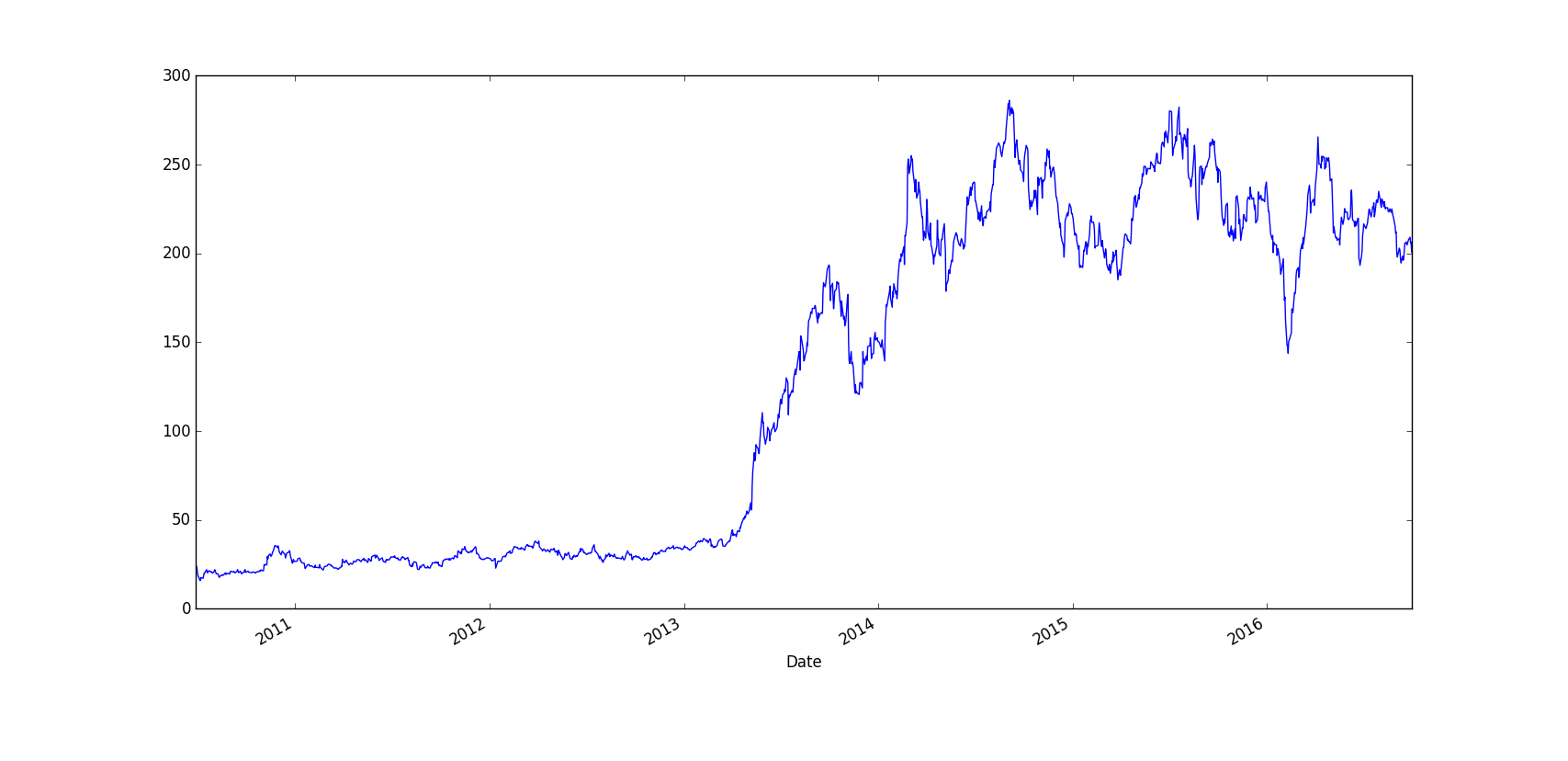
fig,ax = plt.subplots()
TESLA['Close'].plot(figsize=(7,5))
plt.show()
# plot of Tesla's closing prices

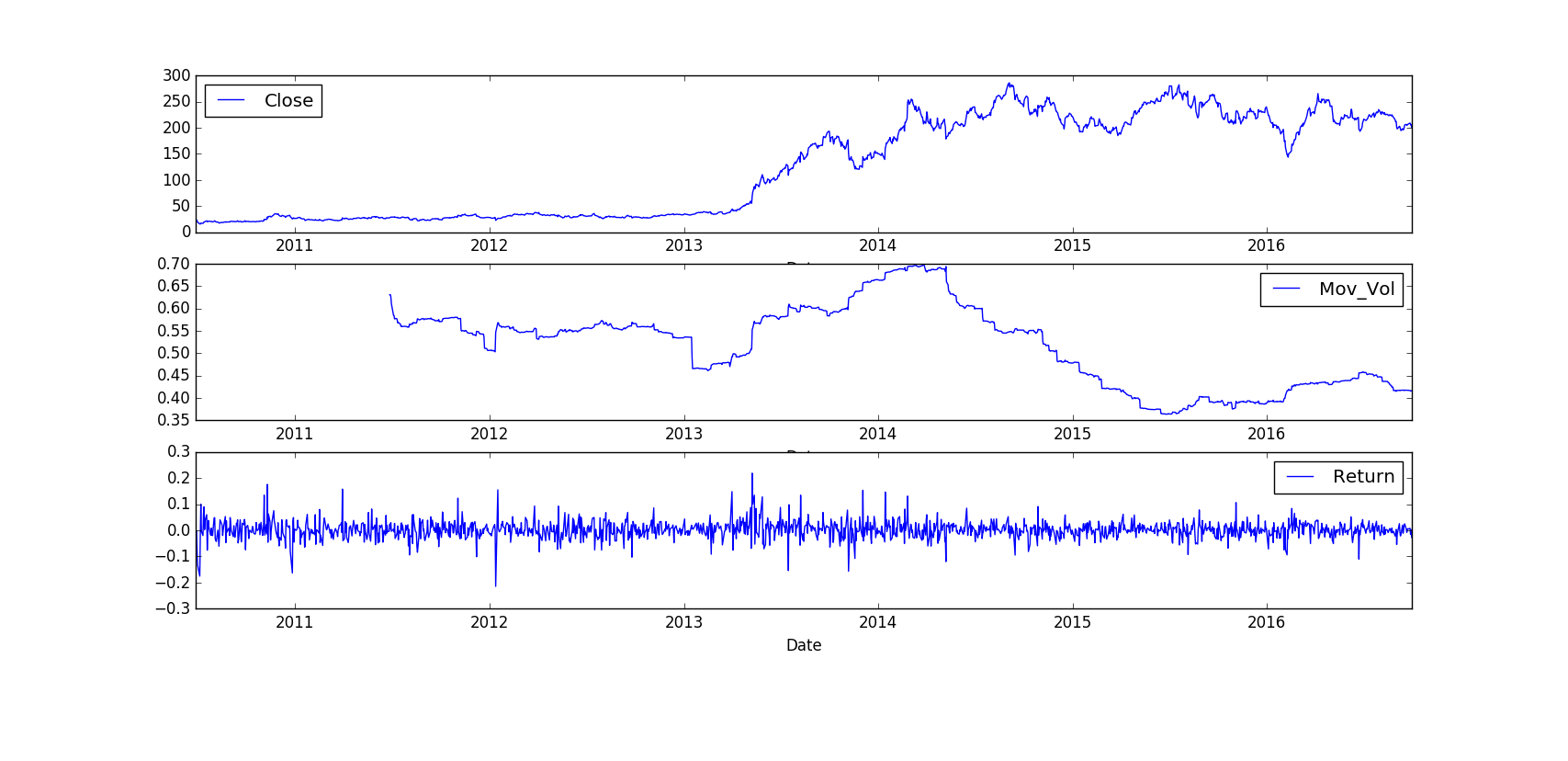
# computing and plotting returns

TESLA['Return'] = np.log(TESLA['Close']/TESLA['Close'].shift(1))
TESLA['42d'] = pd.rolling_mean(TESLA['Close'],window=42)
TESLA['252d'] = pd.rolling_mean(TESLA['Close'],window=252)
TESLA['Mov_Vol'] = pd.rolling_std(TESLA['Return'], window=252)*math.sqrt(252)

# as market goes up volatitiy comes down and vice-versa
TESLA[['Close','Mov_Vol','Return']].plot(ax=ax, subplots=True, style='b', figsize=(8.5))
plt.show()